Methods: Environmental inputs

Modelling Asparagopsis nitrogen bioremediation efficiency in Australian coastal environments

Author

Tormey Reimer

Published

5 August 2026

Cell information

Load in all the BARRA-R2 cells being used, with their coordinates.
cell_coords <- find_read(envi_data, "R2_cell_coords") %>% 
  mutate(state = factor(state, levels = states_ord)) %>% 
  dplyr::select(-layer)
cells_included <- find_read(runs_data, "include")
cells_omitted <- find_read(runs_data, "omit")

totals <- cell_coords %>% 
  filter(!cell_no %in% cells_omitted) %>% 
  group_by(state) %>% 
  reframe(cells = n())

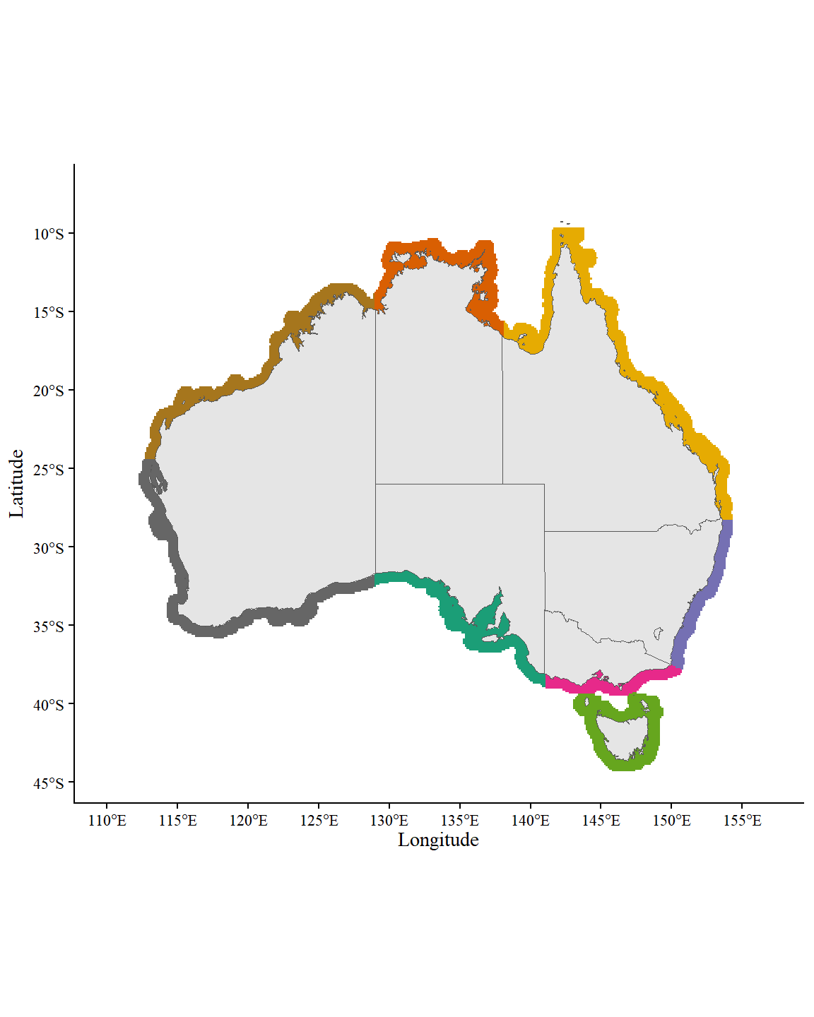
The waters around Australia were divided into 13207 cells for this analysis: 672 in Victoria, 764 in New South Wales, 3005 in Queensland, 1605 in South Australia, 4065 in Western Australia (divided into 1937 cells in the north and 2128 in the south), 1359 in Tasmania, and 1737 in the Northern Territory.

Code
p_cell_map <- cell_coords %>% 
  ggplot(aes(x = longitude, y = latitude, fill = state, label = cell_no)) +
  geom_raster() +
  geom_sf(data = ozmap_data(data = "states"), inherit.aes = F) +
  coord_sf(xlim = c(bounds[["AUS"]]["lonmin"], bounds[["AUS"]]["lonmax"]),
           ylim = c(bounds[["AUS"]]["latmin"], bounds[["AUS"]]["latmax"])) +
  # coord_sf(xlim = c(149.5, 151.5),
  #          ylim = c(-39, -37)) +
  # geom_text(size = 2.25) +
  scale_x_continuous(breaks = seq(100, 160, 5)) +
  scale_y_continuous(breaks = seq(-5, -45, -5)) +
  scale_fill_manual(values = states_pal) +
  labs(x = "Longitude", y = "Latitude") +
  prettyplot() +
  theme(legend.position = "none")

p_cell_map
Figure 1: Map showing the area included this analysis, with colours indicating the different states. The ~60 km coastline buffer includes 95,418 cells approximately 4 x 4 km each.

Environmental inputs

Code
T_input <- file.path(envi_data, "cell_input_all") %>% 
  list.files(full.names = T) %>% 
  purrr::map(function(fnm) {
    fnm %>% arrow::read_parquet(col_select = c("cell_no", "state", "yday", "T_input"))
  }) %>% 
  bind_rows() %>% 
  mutate(state = factor(state, levels = states_ord, labels = states_lng))

(T_means <- T_input %>% 
  group_by(state) %>% 
  reframe(mean = mean(T_input, na.rm = T),
          max = max(T_input, na.rm = T),
          min = min(T_input, na.rm = T)) %>% 
  mutate(variable = "T_input"))
# A tibble: 8 × 5
  state                  mean   max   min variable
  <fct>                 <dbl> <dbl> <dbl> <chr>   
1 Northern Territory     28.7  36.3 20.2  T_input 
2 Queensland             26.6  36.0 12.6  T_input 
3 New South Wales        21.7  33.1  8.07 T_input 
4 South Australia        17.5  32.8  8.14 T_input 
5 Tasmania               15.2  24.0  4.19 T_input 
6 Victoria               16.3  31.3  7.04 T_input 
7 Western Australia (N)  27.8  39.5 16.9  T_input 
8 Western Australia (S)  20.3  37.6  9.44 T_input 
Code
I_input <- file.path(envi_data, "cell_input_all") %>% 
  list.files(full.names = T) %>% 
  purrr::map(function(fnm) {
    fnm %>% arrow::read_parquet(col_select = c("cell_no", "state", "yday", "I_input"))
  }) %>% 
  bind_rows() %>% 
  mutate(state = factor(state, levels = states_ord, labels = states_lng))

(I_means <- I_input %>% 
  group_by(state) %>% 
  reframe(mean = mean(I_input, na.rm = T),
          max = max(I_input, na.rm = T),
          min = min(I_input, na.rm = T)) %>% 
  mutate(variable = "I_input"))
# A tibble: 8 × 5
  state                  mean   max   min variable
  <fct>                 <dbl> <dbl> <dbl> <chr>   
1 Northern Territory     401.  615.  22.4 I_input 
2 Queensland             395.  649.  40.4 I_input 
3 New South Wales        329.  644.  56.6 I_input 
4 South Australia        318.  709.  32.1 I_input 
5 Tasmania               249.  648.  12.5 I_input 
6 Victoria               275.  658.  35.2 I_input 
7 Western Australia (N)  435.  666.  77.1 I_input 
8 Western Australia (S)  357.  715.  28.6 I_input 
Code
K_input <- file.path(envi_data, "cell_input_all") %>% 
  list.files(full.names = T) %>% 
  purrr::map(function(fnm) {
    fnm %>% arrow::read_parquet(col_select = c("cell_no", "state", "yday", "Kd_490"))
  }) %>% 
  bind_rows() %>% 
  mutate(state = factor(state, levels = states_ord, labels = states_lng))

(K_means <- K_input %>% 
  group_by(state) %>% 
  reframe(mean = mean(Kd_490, na.rm = T),
          max = max(Kd_490, na.rm = T),
          min = min(Kd_490, na.rm = T)) %>% 
  mutate(variable = "Kd_490"))
# A tibble: 8 × 5
  state                   mean   max    min variable
  <fct>                  <dbl> <dbl>  <dbl> <chr>   
1 Northern Territory    0.132   6.00 0.0188 Kd_490  
2 Queensland            0.107   6.00 0.0169 Kd_490  
3 New South Wales       0.0983  6.00 0.0172 Kd_490  
4 South Australia       0.124   6.00 0.0172 Kd_490  
5 Tasmania              0.108   6.00 0.0182 Kd_490  
6 Victoria              0.165   6.00 0.0196 Kd_490  
7 Western Australia (N) 0.111   6.00 0.0176 Kd_490  
8 Western Australia (S) 0.0627  6.00 0.0176 Kd_490  
Code
S_input <- file.path(envi_data, "cell_input_all") %>% 
  list.files(full.names = T) %>% 
  purrr::map(function(fnm) {
    fnm %>% arrow::read_parquet(col_select = c("cell_no", "state", "yday", "S_input"))
  }) %>% 
  bind_rows() %>% 
  mutate(state = factor(state, levels = states_ord, labels = states_lng))

(S_means <- S_input %>% 
  group_by(state) %>% 
  reframe(mean = mean(S_input, na.rm = T),
          max = max(S_input, na.rm = T),
          min = min(S_input, na.rm = T)) %>% 
  mutate(variable = "S_input"))
# A tibble: 8 × 5
  state                  mean   max   min variable
  <fct>                 <dbl> <dbl> <dbl> <chr>   
1 Northern Territory     34.5  35.6  32.8 S_input 
2 Queensland             34.9  35.9  32.7 S_input 
3 New South Wales        35.5  35.7  35.1 S_input 
4 South Australia        35.9  37.2  35.2 S_input 
5 Tasmania               35.4  35.7  35.0 S_input 
6 Victoria               35.5  35.8  35.3 S_input 
7 Western Australia (N)  35.0  35.9  34.2 S_input 
8 Western Australia (S)  35.7  36.4  35.0 S_input 
Code
UV_input <- file.path(envi_data, "cell_input_all") %>% 
  list.files(full.names = T) %>% 
  purrr::map(function(fnm) {
    fnm %>% arrow::read_parquet(col_select = c("cell_no", "state", "yday", "UV_input"))
  }) %>% 
  bind_rows() %>% 
  mutate(state = factor(state, levels = states_ord, labels = states_lng))

(UV_means <- UV_input %>% 
  group_by(state) %>% 
  reframe(mean = mean(UV_input, na.rm = T),
          max = max(UV_input, na.rm = T),
          min = min(UV_input, na.rm = T)) %>% 
  mutate(variable = "UV_input"))
# A tibble: 8 × 5
  state                   mean   max       min variable
  <fct>                  <dbl> <dbl>     <dbl> <chr>   
1 Northern Territory    0.0573 0.348 0.0000610 UV_input
2 Queensland            0.124  1.06  0.0000440 UV_input
3 New South Wales       0.349  1.46  0.000463  UV_input
4 South Australia       0.0702 0.681 0.0000782 UV_input
5 Tasmania              0.0835 0.617 0.0000366 UV_input
6 Victoria              0.0892 0.791 0.000220  UV_input
7 Western Australia (N) 0.0663 0.559 0.000113  UV_input
8 Western Australia (S) 0.124  0.843 0.000116  UV_input

Mean daily temperature ranged from 15.2 in Tasmania to 28.7 in Northern Territory, with a mean across states of 21.8.

Code
T_input_state <- T_input %>%
  group_by(state, yday) %>% 
  reframe(value = mean(T_input, na.rm = T),
          sd = sd(T_input, na.rm = T))

(
  p_input_state_av <- T_input_state %>% 
    ggplot(aes(x = yday, y = value, ymin = value-sd, ymax = value+sd, colour = state, fill = state)) +
    geom_line(linewidth = 0.75) +
    geom_ribbon(alpha = 0.35, linewidth = 0.25) +
    facet_wrap(facets = vars(state), ncol = 2) +
    scale_y_continuous(breaks = seq(0, 40, 5), limits = c(10, 35)) +
    scale_colour_manual(values = states_pal) +
    scale_fill_manual(values = states_pal) +
    env_plot() +
    labs(x = "Day of the year", y = expression("Temperature ("*degree*"C)"))
)
Figure 2: Summary of temperature values across the year within each state, averaged across 2019-2023. Bold lines show the mean across all cells within each state while ribbons show the standard deviation between cells.

Mean daily irradiance ranged from 249 in Tasmania to 435 in Western Australia (N), with a mean across states of 345.

Code
I_input_state <- I_input %>%
  group_by(state, yday) %>% 
  reframe(value = mean(I_input, na.rm = T),
          sd = sd(I_input, na.rm = T))

p_input_state_av %+% I_input_state +
  scale_y_continuous(breaks = seq(0, 1600, 150), limits = c(0, 650)) +
  labs(x = "Day of the year", y = expression("Irradiance (photons m"^-2*" s"^-1*")")) 
Warning: <ggplot> %+% x was deprecated in ggplot2 4.0.0.
ℹ Please use <ggplot> + x instead.
Scale for y is already present.
Adding another scale for y, which will replace the existing scale.
Warning: Removed 1 row containing missing values or values outside the scale range
(`geom_ribbon()`).
Figure 3: Summary of irradiance values across the year within each state, averaged across 2019-2023. Bold lines show the mean across all cells within each state while ribbons show the standard deviation between cells.

Mean daily values for the light attenuation coefficient in water ranged from 6.27 \(\times 10^2\) in Western Australia (S) to 1.65 \(\times 10\) in Victoria, with a mean across states of 11.33 \(\times 10^2\).

Code
K_input_state <- K_input %>%
  group_by(state, yday) %>% 
  reframe(value = mean(Kd_490, na.rm = T),
          sd = sd(Kd_490, na.rm = T)) %>% 
  mutate(sd = case_when(sd > value ~ value, T ~ sd))

p_input_state_av %+% K_input_state +
  scale_y_continuous(breaks = seq(0, 0.7, 0.1), limits = c(0, 0.62)) +
  labs(x = "Day of the year", y = expression("Light attenuation coefficient (m"^-1*" )"))
Scale for y is already present.
Adding another scale for y, which will replace the existing scale.
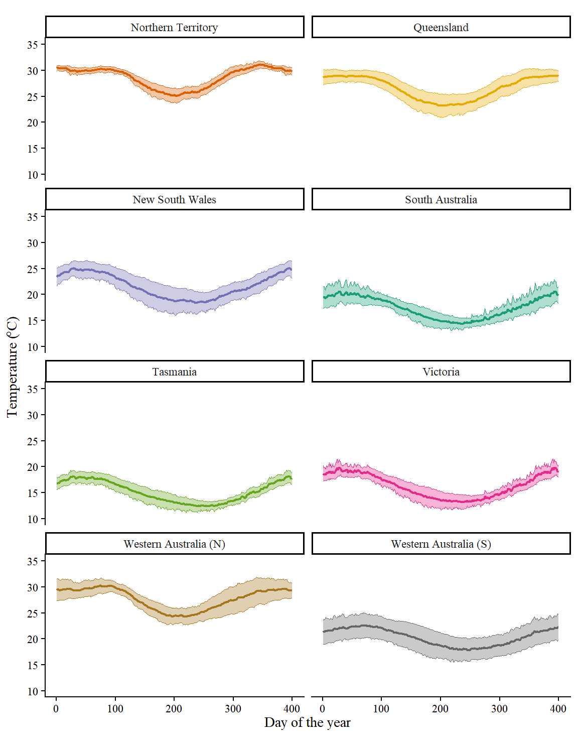
Figure 4: Summary of irradiance values across the year within each state, averaged across 2019-2023. Bold lines show the mean across all cells within each state while ribbons show the standard deviation between cells.

Mean daily salinity ranged from 34.5 in Northern Territory to 35.9 in South Australia, with a mean across states of 35.3.

Code
S_input_state <- S_input %>%
  group_by(state, yday) %>% 
  reframe(value = mean(S_input, na.rm = T),
          sd = sd(S_input, na.rm = T))

p_input_state_av %+% S_input_state +
  scale_y_continuous(breaks = seq(30, 40, 0.5), limits = c(33.85, 36.5)) +
  labs(x = "Day of the year", y = expression("Salinity (g L"^-1*")"))
Scale for y is already present.
Adding another scale for y, which will replace the existing scale.
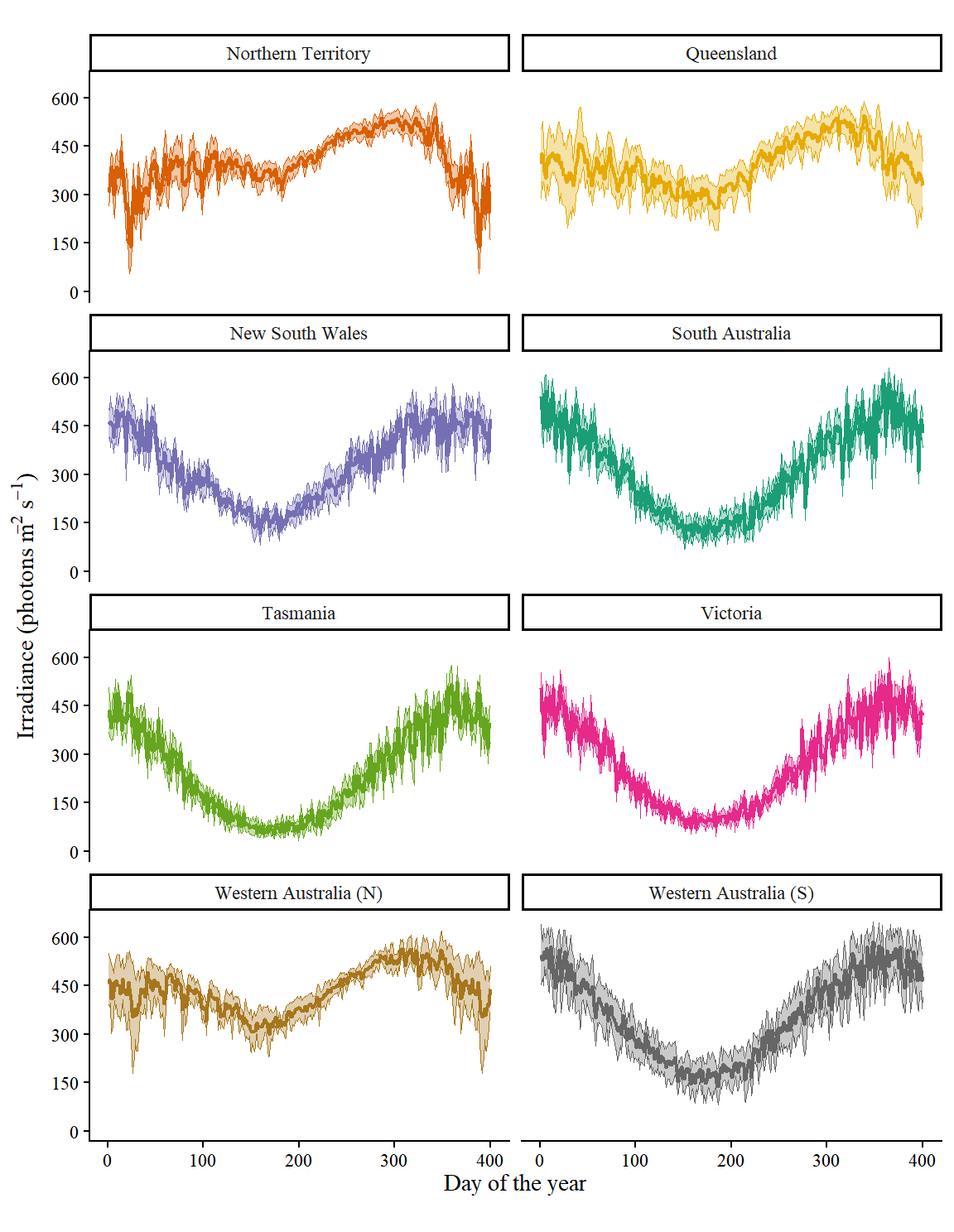
Figure 5: Summary of salinity values across the year within each state, averaged across 2019-2023 and all depths < 25 m. Bold lines show the mean across all cells within each state while ribbons show the standard deviation between cells.

Mean daily water velocity ranged from 0.06 in Northern Territory to 0.35 in New South Wales, with a mean across states of 0.12.

Code
UV_input_state <- UV_input %>%
  group_by(state, yday) %>% 
  reframe(value = mean(UV_input, na.rm = T),
          sd = sd(UV_input, na.rm = T)) %>% 
  mutate(sd_min = case_when(sd > value ~ value, T ~ sd))

(
  p_input_state_av <- UV_input_state %>% 
    ggplot(aes(x = yday, y = value, ymin = value-sd_min, ymax = value+sd, colour = state, fill = state)) +
    geom_line(linewidth = 0.75) +
    geom_ribbon(alpha = 0.35, linewidth = 0.25) +
    facet_wrap(facets = vars(state), ncol = 2) +
    scale_y_continuous(breaks = seq(0, 1, 0.2), limits = c(-0.01, 1)) +
    scale_colour_manual(values = states_pal) +
    scale_fill_manual(values = states_pal) +
    env_plot() +
    labs(x = "Day of the year", y = expression("Water velocity (m s"^-1*")"))
)
Figure 6: Summary of water velocity values across the year within each state, averaged across 2019-2023 and all depths < 25 m. Bold lines show the mean across all cells within each state while ribbons show the standard deviation between cells.

Ambient nitrogen

Code
refstation_locations <- here() %>% 
  file.path("data", "nitrogen", "refstation_locations.parquet") %>% 
  arrow::read_parquet() %>% 
  rename(name = StationName) %>% 
  dplyr::select(-code)

outfall_locations <- here() %>% 
  file.path("data_raw", "national-outfall-database", "data-output", "outflow_site_locations.parquet") %>% 
  arrow::read_parquet() %>% 
  rename(lon = longitude,
         lat = latitude) %>% 
  dplyr::select(-state)

N_locations <- rbind(
  outfall_locations %>% mutate(type = "outfall"),
  refstation_locations %>% mutate(type = "refstation")
) %>% 
  mutate(name = as.character(name),
         state = case_when(
    lon > bounds[["SAU"]]["lonmin"] & lon <= bounds[["SAU"]]["lonmax"] & 
      lat > bounds[["SAU"]]["latmin"] & lat <= bounds[["SAU"]]["latmax"]  ~ "SAU",
    lon > bounds[["QLD"]]["lonmin"] & lon <= bounds[["QLD"]]["lonmax"] & 
      lat > bounds[["QLD"]]["latmin"] & lat <= bounds[["QLD"]]["latmax"]  ~ "QLD",
    lon > bounds[["WAS"]]["lonmin"] & lon <= bounds[["WAS"]]["lonmax"] & 
      lat > bounds[["WAS"]]["latmin"] & lat <= bounds[["WAS"]]["latmax"]  ~ "WAS",
    lon > bounds[["WAN"]]["lonmin"] & lon <= bounds[["WAN"]]["lonmax"] & 
      lat > bounds[["WAN"]]["latmin"] & lat <= bounds[["WAN"]]["latmax"]  ~ "WAN",
    lon > bounds[["VIC"]]["lonmin"] & lon <= bounds[["VIC"]]["lonmax"] & 
      lat > bounds[["VIC"]]["latmin"] & lat <= bounds[["VIC"]]["latmax"]  ~ "VIC",
    lon > bounds[["NSW"]]["lonmin"] & lon <= bounds[["NSW"]]["lonmax"] & 
      lat > bounds[["NSW"]]["latmin"] & lat <= bounds[["NSW"]]["latmax"]  ~ "NSW",
    lon > bounds[["NTE"]]["lonmin"] & lon <= bounds[["NTE"]]["lonmax"] & 
      lat > bounds[["NTE"]]["latmin"] & lat <= bounds[["NTE"]]["latmax"]  ~ "NTE",
    lon > bounds[["TAS"]]["lonmin"] & lon <= bounds[["TAS"]]["lonmax"] & 
      lat > bounds[["TAS"]]["latmin"] & lat <= bounds[["TAS"]]["latmax"]  ~ "TAS",
    TRUE ~ NA
  ),
  state = factor(state, levels = states_ord)) %>% 
  relocate(state, .before = name) %>% 
  rename(latitude = lat,
         longitude = lon)

refstation_locations <- filter(N_locations, type == "refstation")
outfall_locations <- filter(N_locations, type == "outfall")
Code
ggplot(N_locations, aes(x = longitude, y = latitude, color = state, shape = type)) +
  geom_sf(data = ozmap_data(data = "states"), inherit.aes = F) +
  coord_sf(xlim = c(bounds[["AUS"]]["lonmin"], bounds[["AUS"]]["lonmax"]),
           ylim = c(bounds[["AUS"]]["latmin"], bounds[["AUS"]]["latmax"])) +
  geom_point(size = 3.5) +
  scale_shape_manual(values = c(20, 13)) +
  # scale_colour_manual(values = states_pal, labels = states_lng, na.value = "black") +
  scale_color_manual(values = states_pal) +
  scale_x_continuous(breaks = seq(100, 160, 5)) +
  scale_y_continuous(breaks = seq(-5, -45, -5)) +
  labs(x = "Longitude", y = "Latitude") +
  prettyplot() +
  theme(legend.position = "none")
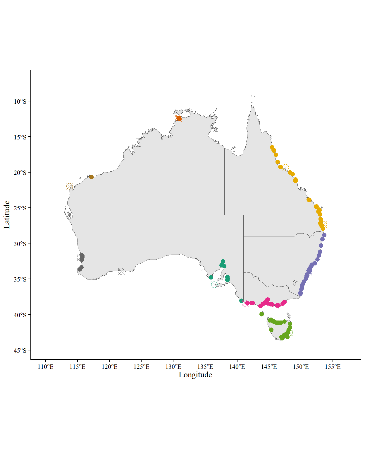
Figure 7: Map showing the locations of recorded outfalls (points, coloured by state) and the IMOS reference stations (stars) used in this analysis.
Code
all_cells <- sum(totals$cells)

cells_by_station <- file.path(envi_data, "N_data_cells_bystation.parquet") %>% read_parquet()
cells_by_station_1 <- cells_by_station %>% 
  filter(data_source == "refstation") %>% 
  mutate(name = droplevels(name))
cells_by_station_2 <- cells_by_station %>% filter(data_source != "refstation")
stations_by_cell <- file.path(envi_data, "N_data_stations_bycell.parquet") %>% read_parquet()
stations_by_cell_1 <- stations_by_cell %>% filter(data_source == "refstation")
stations_by_cell_2 <- stations_by_cell %>% filter(data_source != "refstation")

# levels(cells_by_station_1$name)

Matching model cells to their two nearest reference stations resulted in 41% of cells using data from Darwin, 31% using data from Kangaroo Island, 24.1% using data from Maria Island, 16% from North Stradbroke Island, 20.5% using data from Port Hacking, 31.4% using data from Rottnest Island, and 36% using data from Yongala.

There were 8 outfall stations in South Australia, 9 in southern Western Australia, 1 in northern Western Australia, 32 in southern New South Wales, 29 in Queensland, 18 in Victoria, 32 in Tasmania, and 4 in the Northern Territory.

Matching cells to outfall stations within 48 km resulted in 7% of cells using data from one outfall site, 4.9% of cells using data from two or three sites, 1.3% of cells using data from three or four sites, 0.6% of cells using data from six to eight sites, and 0.2% of cells using data from nine to twelve sites. The remaining 86.1% of cells did not use data from any outfall sites.

Code
# stations_by_cell %>% filter(data_source != "refstation" & num>=2) %>% merge(cell_coords, by = "cell_no") %>% filter(state == "NSW") %>% pull(cell_no) %>% sample(size = 1)
eg_cell <- 108843

BARRA_R2_cell_nos <- file.path(envi_data, "BARRA_R2_cell_nos.qs") %>% qs::qread()
ind <- which(BARRA_R2_cell_nos == eg_cell)

N_data <- find_read(file.path(envi_data, "combined_N_data"), "N_data_combined") %>% 
  filter(cell_no == eg_cell) %>% 
  mutate(value = value %>% set_units("mg m-3") %>% set_units("umol L-1") %>% drop_units())

N_curve <- find_read(file.path(envi_data, "combined_N_data"), "parameter") %>% 
  filter(cell_no == eg_cell) 
N_curve <- data.frame(yday = 1:365) %>% 
  mutate(ammonia = N_curve$a[N_curve$measure == "Am"] + N_curve$b[N_curve$measure == "Am"] * 
           sin((yday * pi + N_curve$c[N_curve$measure == "Am"]) / 182.5),
         nitrate_nitrite = N_curve$a[N_curve$measure == "Ni"] + N_curve$b[N_curve$measure == "Ni"] * 
           sin((yday * pi + N_curve$c[N_curve$measure == "Ni"]) / 182.5)) %>% 
  pivot_longer(names_to = "indicator", values_to = "value", cols = c("ammonia", "nitrate_nitrite"), 
               names_transform = list(indicator = as.factor)) %>% 
  mutate(value = value %>% set_units("mg m-3") %>% set_units("umol L-1"))

N_input <- file.path(envi_data, "cell_input_all") %>% 
  list.files(full.names = T) %>% 
  purrr::map(function(fnm){
    read_parquet(fnm) %>% 
      filter(cell_no == eg_cell)
  }) %>% 
  bind_rows() %>% 
  select(yday, Ni_input, Am_input) %>% 
  pivot_longer(names_to = "indicator", values_to = "value", cols = c("Ni_input", "Am_input"), 
               names_transform = list(indicator = as.factor)) %>% 
  mutate(value = value %>% set_units("mg m-3") %>% set_units("umol L-1") %>% drop_units(),
         indicator = factor(indicator, levels = c("Am_input", "Ni_input"), labels = levels(N_data$indicator)))

ggplot(N_data, aes(x = yday, y = value, fill = data_source, colour = data_source, size = weight)) +
  geom_point(shape = 21, alpha = 0.15) +
  facet_wrap(facets = vars(indicator), nrow = 2, scales = "free") +
  geom_line(data = N_input, aes(x = yday, y = value), inherit.aes = F) +
  scale_fill_manual(values = c("steelblue", "orange")) +
  scale_colour_manual(values = c("steelblue", "orange")) +
  # scale_y_continuous(limits = c(0, 3.5), breaks = seq(0, 4, 0.5)) +
  env_plot() +
  theme(strip.text = element_blank(), aspect.ratio = 0.55) +
  scale_x_continuous(breaks = seq(0,360,60)) +
  labs(x = "Day of the year", y = nitrogen_lab)
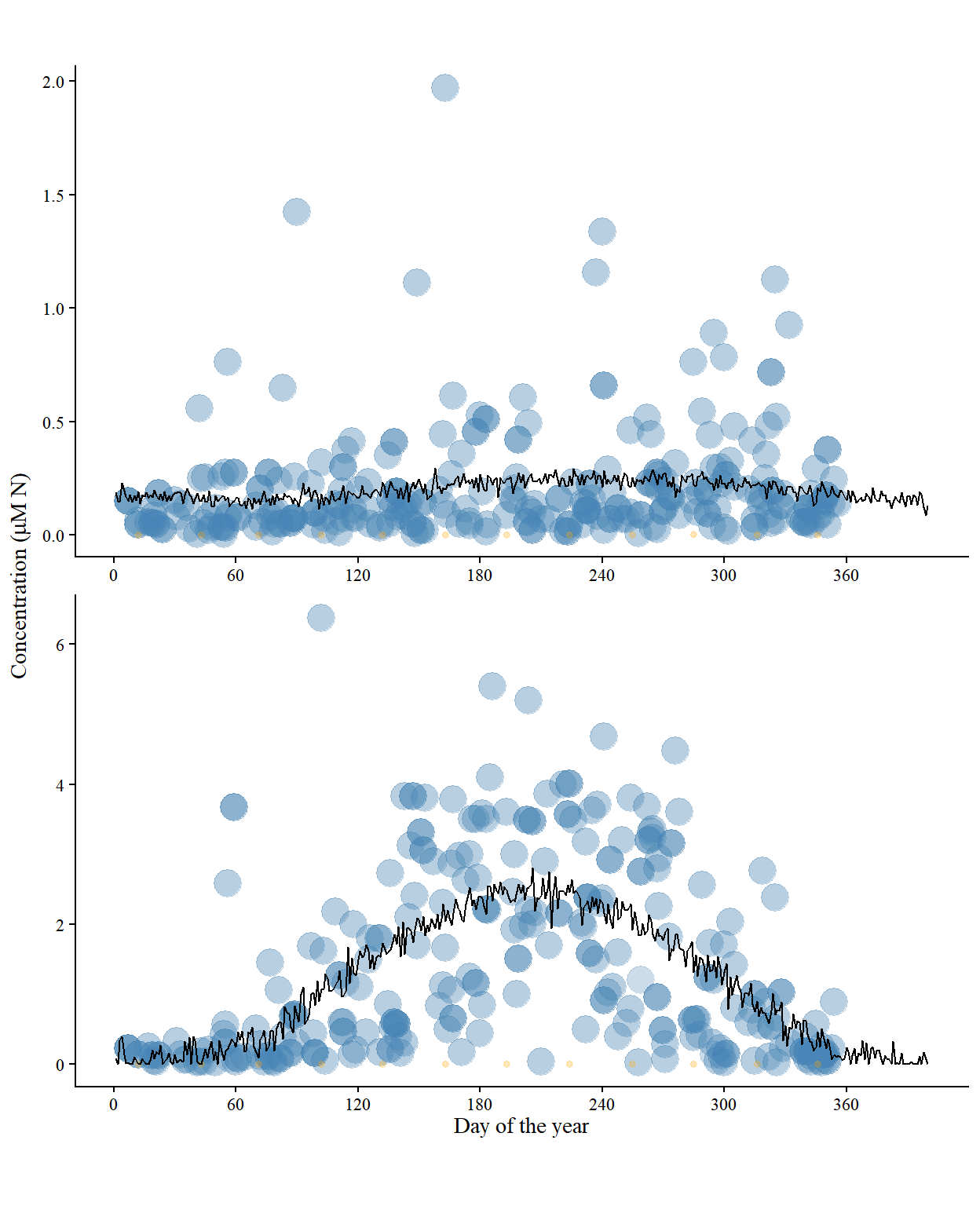
Figure 8: An example of the daily nitrate (top) and ammonium (bottom) input and data for a single cell in New South Wales. Black lines show the input driving the growth model (constructed curve), blue dots show data from the nearest reference station (Port Hacking) and orange dots show distance-weighted data from the three nearest outfall points (Bateman’s Bay, Bermagui, and Bombo).
Code
Ni_input <- file.path(envi_data, "cell_input_all") %>% 
  list.files(full.names = T) %>% 
  purrr::map(function(fnm) {
    fnm %>% arrow::read_parquet(col_select = c("cell_no", "state", "yday", "Ni_input"))
  }) %>% 
  bind_rows() %>% 
  mutate(state = factor(state, levels = states_ord, labels = states_lng)) %>% 
  mutate(Ni_input = Ni_input %>% set_units("mg m-3") %>% set_units("umol L-1"))

(Ni_means <- Ni_input %>% 
  group_by(state) %>% 
  reframe(mean = mean(Ni_input, na.rm = T),
          max = max(Ni_input, na.rm = T),
          min = min(Ni_input, na.rm = T)) %>% 
  mutate(variable = "Ni_input"))
# A tibble: 8 × 5
  state                     mean      max      min variable
  <fct>                 [umol/L] [umol/L] [umol/L] <chr>   
1 Northern Territory       0.417    1.03         0 Ni_input
2 Queensland               0.302    1.22         0 Ni_input
3 New South Wales          0.705    3.07         0 Ni_input
4 South Australia          0.939    3.31         0 Ni_input
5 Tasmania                 1.20     3.26         0 Ni_input
6 Victoria                 1.20     3.24         0 Ni_input
7 Western Australia (N)    0.372    1.02         0 Ni_input
8 Western Australia (S)    0.205    0.915        0 Ni_input
Code
Ni_input %>% 
  pull(Ni_input) %>% 
  max()
3.314379 [umol/L]
Code
(3.314379 + 3.5)/3.314379
[1] 2.056005

Mean daily water velocity ranged from 0.21 in Western Australia (S) to 1.2 in Victoria, with a mean across states of 0.67.

Code
Ni_input_state <- Ni_input %>%
  group_by(state, yday) %>% 
  reframe(value = mean(Ni_input, na.rm = T),
          sd = sd(Ni_input, na.rm = T)) %>% 
  mutate(value = value %>% drop_units())

(
  p_input_state_av <- Ni_input_state %>% 
    ggplot(aes(x = yday, y = value, ymin = value-sd, ymax = value+sd, colour = state, fill = state)) +
    geom_line(linewidth = 0.75) +
    geom_ribbon(alpha = 0.35, linewidth = 0.25) +
    facet_wrap(facets = vars(state), ncol = 2) +
    # scale_y_continuous(breaks = seq(0, 40, 5), limits = c(10, 35)) +
    scale_colour_manual(values = states_pal) +
    scale_fill_manual(values = states_pal) +
    env_plot() +
    labs(x = "Day of the year", y = nitrate_lab)
)
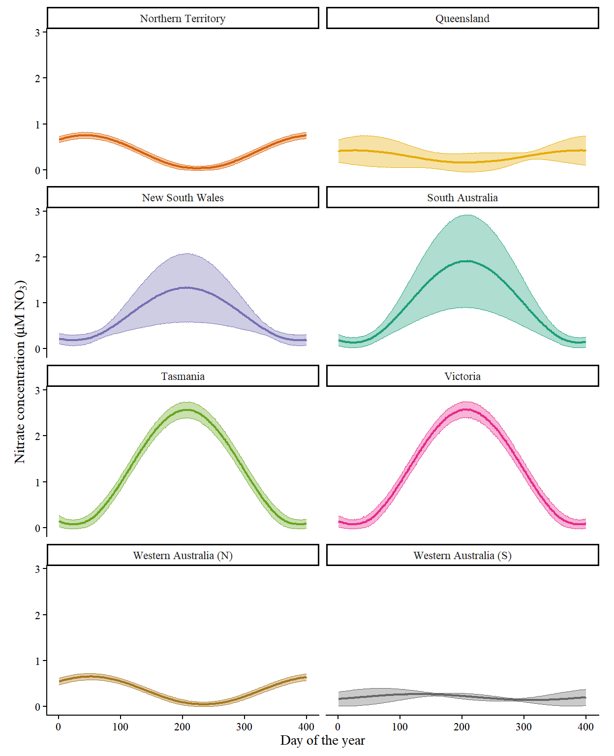
Figure 9: Summary of nitrate concentration values across the year within each state, averaged across 2019-2023. Bold lines show the mean across all cells within each state while ribbons show the standard deviation between cells.
Code
Am_input <- file.path(envi_data, "cell_input_all") %>% 
  list.files(full.names = T) %>% 
  purrr::map(function(fnm) {
    fnm %>% arrow::read_parquet(col_select = c("cell_no", "state", "yday", "Am_input"))
  }) %>% 
  bind_rows() %>% 
  mutate(state = factor(state, levels = states_ord, labels = states_lng)) %>% 
  mutate(Am_input = Am_input %>% set_units("mg m-3") %>% set_units("umol L-1"))

(Am_means <- Am_input %>% 
  group_by(state) %>% 
  reframe(mean = mean(Am_input, na.rm = T),
          max = max(Am_input, na.rm = T),
          min = min(Am_input, na.rm = T)) %>% 
  mutate(variable = "Am_input"))
# A tibble: 8 × 5
  state                     mean      max      min variable
  <fct>                 [umol/L] [umol/L] [umol/L] <chr>   
1 Northern Territory       0.150    0.259 0.0288   Am_input
2 Queensland               0.159    0.405 0.00858  Am_input
3 New South Wales          0.232    0.411 0.0658   Am_input
4 South Australia          0.180    0.424 0.000844 Am_input
5 Tasmania                 0.189    0.356 0.0179   Am_input
6 Victoria                 0.189    0.439 0.00696  Am_input
7 Western Australia (N)    0.151    0.269 0.0223   Am_input
8 Western Australia (S)    0.129    0.264 0.0294   Am_input
Code
Am_input %>% 
  pull(Am_input) %>% 
  max()
0.4390794 [umol/L]
Code
(0.4390794 + 6.5)/0.4390794
[1] 15.8037
Code
supp_times <- list()
for (st in 1:8) {
  state <- levels(Am_input$state)[st]
  supp_times[[st]] <- rbind(
    Am_input %>% 
      filter(state == state) %>% 
      rename(value = Am_input) %>% 
      mutate(value = drop_units(value), supp_value = value + 6.5), 
    Ni_input %>% 
      filter(state == state) %>% 
      rename(value = Ni_input) %>% 
      mutate(value = drop_units(value), supp_value = value + 6.5)
  ) %>% 
    group_by(cell_no, yday) %>% 
    reframe(
      value = sum(value, na.rm = T),
      supp_value = sum(supp_value, na.rm = T)
    ) %>% 
    mutate(times = supp_value/value)
}
supp_times <- bind_rows(supp_times)

max(supp_times$times)
[1] 412.7134
Code
mean(supp_times$times)
[1] 34.97192

Mean daily water velocity ranged from 0.13 in Western Australia (S) to 0.23 in New South Wales, with a mean across states of 0.17.

Code
Am_input_state <- Am_input %>%
  group_by(state, yday) %>% 
  reframe(value = mean(Am_input, na.rm = T),
          sd = sd(Am_input, na.rm = T)) %>% 
  mutate(value = value %>% drop_units())

p_input_state_av %+% Am_input_state +
  # scale_y_continuous(breaks = seq(30, 40, 0.5), limits = c(34, 36.5)) +
  labs(x = "Day of the year", y = ammonium_lab)
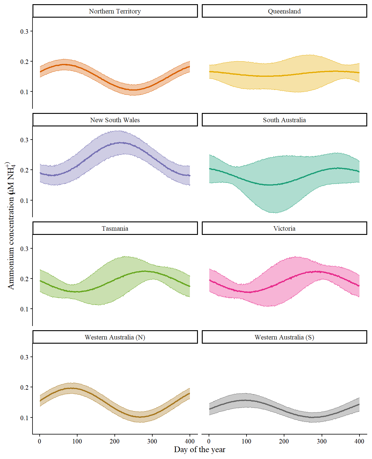
Figure 10: Summary of ammonium concentration values across the year within each state, averaged across 2019-2023. Bold lines show the mean across all cells within each state while ribbons show the standard deviation between cells.

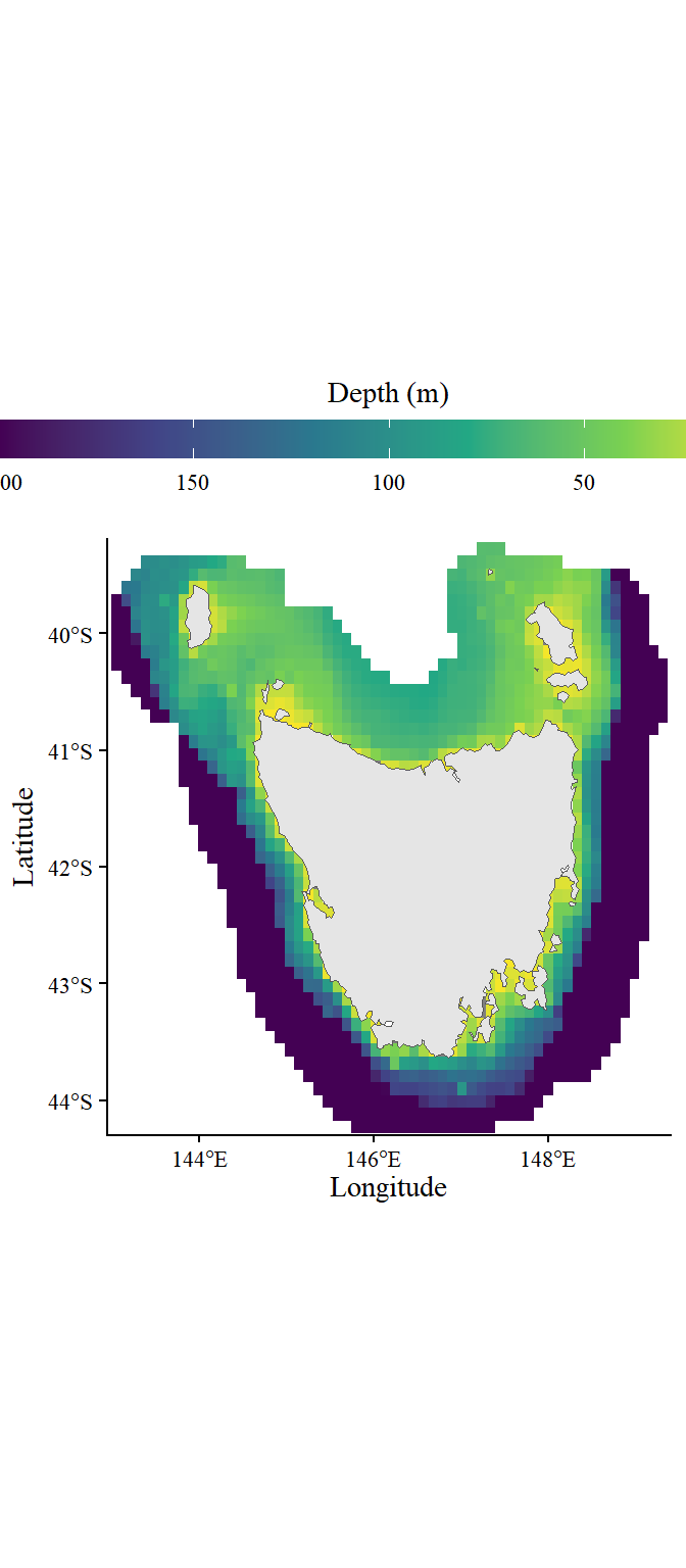
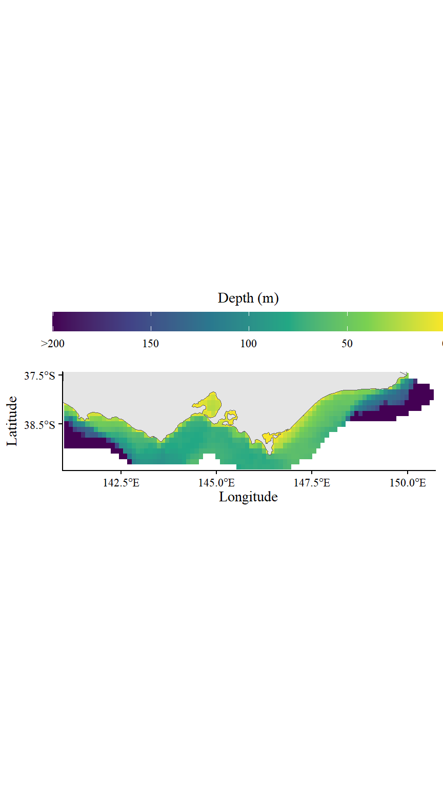
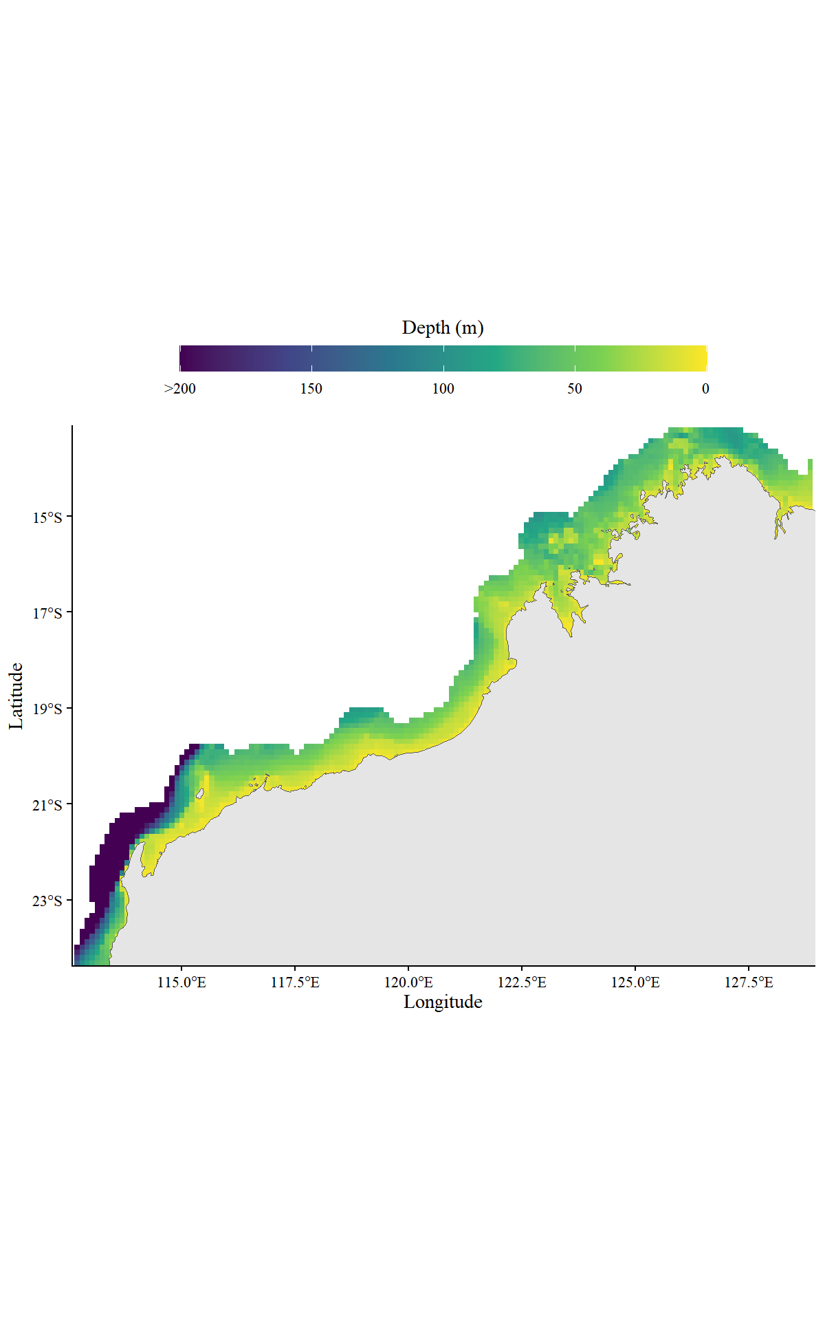
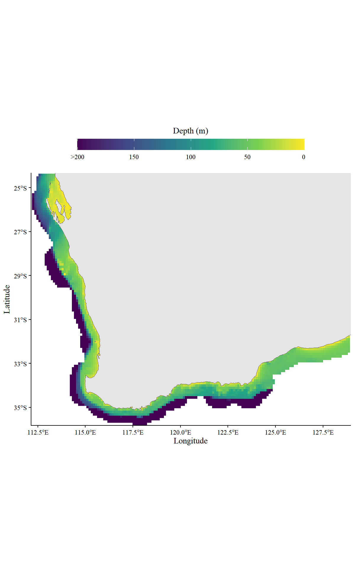
Cell bathymetry

Code
cell_bathy <- file.path(envi_data, "cell_bathy.parquet") %>% 
  arrow::read_parquet() %>% 
  rename(bathy = hz) %>% 
  mutate(bathy = -bathy,
         bathy = case_when(bathy <= -200 ~ -200, TRUE ~ bathy)) %>% 
  merge(cell_coords, by = "cell_no")

lims <- cell_bathy %>% 
  group_by(state) %>% 
  reframe(lonmin = min(longitude)-0.1, 
          lonmax = max(longitude)+0.1,
          latmin = min(latitude)-0.075,
          latmax = max(latitude)+0.075) %>% 
  mutate(widest = max(lonmax-lonmin),
         width = round((lonmax-lonmin)/widest * 6.25, 2),
         minheight = width * (latmax-latmin)/(lonmax-lonmin))
Code
stlims <- lims[lims$state == "NTE", ]

p_bathy <- ggplot(filter(cell_bathy, state == "NTE"), aes(x = longitude, y = latitude, fill = bathy)) +
  geom_raster() +
  geom_sf(data = ozmap_data(data = "states"), inherit.aes = F) +
  coord_sf(xlim = c(stlims$lonmin, stlims$lonmax), ylim = c(stlims$latmin, stlims$latmax), expand = F) +
  scale_x_continuous(breaks = seq(100, 160, 2.5)) +
  scale_y_continuous(breaks = seq(-5, -45, -2)) +
  scale_fill_viridis_c(limits = c(-200, 0), 
                       breaks = seq(0, -200, -50), labels = c("0", "50", "100", "150", ">200"),
                       guide = guide_colorbar(
                         title = "Depth (m)", 
                         barheight = 1, barwidth = 20,
                         title.position = "top",
                         title.hjust = 0.5
                       )) +
  labs(x = "Longitude", y = "Latitude") +
  prettyplot() +
  theme(legend.position = "top")
p_bathy
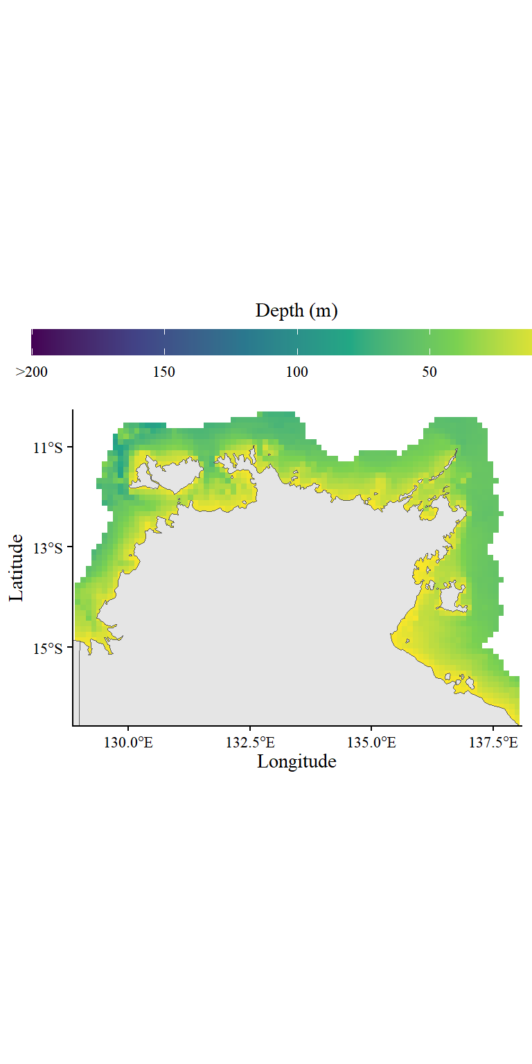
Figure 11
Code
stlims <- lims[lims$state == "QLD", ]

p_bathy %+% filter(cell_bathy, state == "QLD") +
  coord_sf(xlim = c(stlims$lonmin, stlims$lonmax), ylim = c(stlims$latmin, stlims$latmax), expand = F) +
  scale_x_continuous(breaks = seq(100, 160, 5)) +
  scale_y_continuous(breaks = seq(-5, -45, -2.5))
Coordinate system already present.
ℹ Adding new coordinate system, which will replace the existing one.
Scale for x is already present.
Adding another scale for x, which will replace the existing scale.
Scale for y is already present.
Adding another scale for y, which will replace the existing scale.
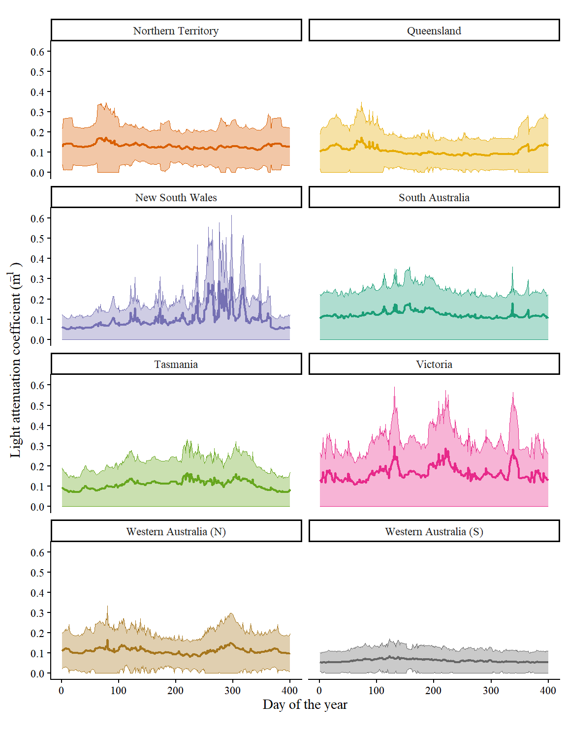
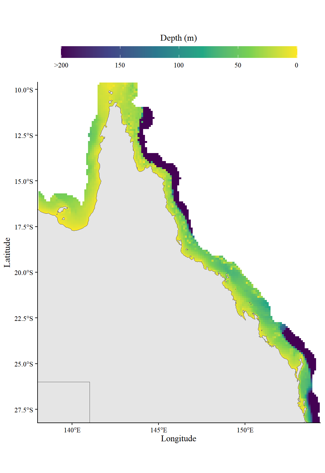
Figure 12
Code
stlims <- lims[lims$state == "NSW", ]

p_bathy %+% filter(cell_bathy, state == "NSW") +
  coord_sf(xlim = c(stlims$lonmin, stlims$lonmax), ylim = c(stlims$latmin, stlims$latmax), expand = F)
Coordinate system already present.
ℹ Adding new coordinate system, which will replace the existing one.
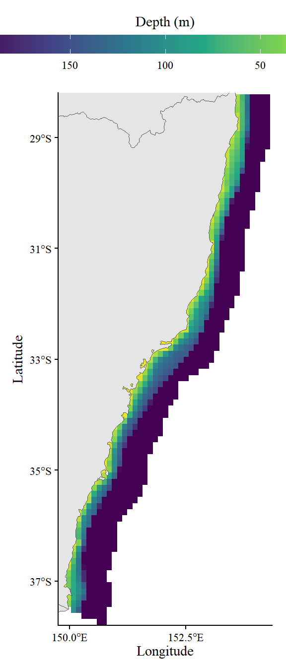
Figure 13
Code
stlims <- lims[lims$state == "SAU", ]

p_bathy %+% filter(cell_bathy, state == "SAU") +
  coord_sf(xlim = c(stlims$lonmin, stlims$lonmax), ylim = c(stlims$latmin, stlims$latmax), expand = F)
Coordinate system already present.
ℹ Adding new coordinate system, which will replace the existing one.
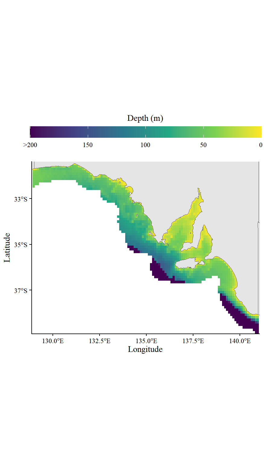
Figure 14
Code
stlims <- lims[lims$state == "TAS", ]

p_bathy %+% filter(cell_bathy, state == "TAS") +
  coord_sf(xlim = c(stlims$lonmin, stlims$lonmax), ylim = c(stlims$latmin, stlims$latmax), expand = F) +
    scale_x_continuous(breaks = seq(100, 160, 2)) +
    scale_y_continuous(breaks = seq(-5, -45, -1))
Coordinate system already present.
ℹ Adding new coordinate system, which will replace the existing one.
Scale for x is already present.
Adding another scale for x, which will replace the existing scale.
Scale for y is already present.
Adding another scale for y, which will replace the existing scale.
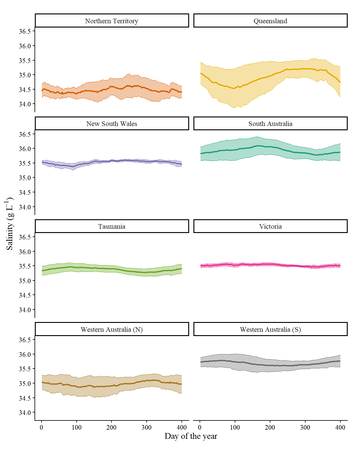
Figure 15
Code
stlims <- lims[lims$state == "VIC", ]

p_bathy %+% filter(cell_bathy, state == "VIC") +
  coord_sf(xlim = c(stlims$lonmin, stlims$lonmax), ylim = c(stlims$latmin, stlims$latmax), expand = F) +
    scale_y_continuous(breaks = seq(-5.5, -45, -1))
Coordinate system already present.
ℹ Adding new coordinate system, which will replace the existing one.
Scale for y is already present.
Adding another scale for y, which will replace the existing scale.
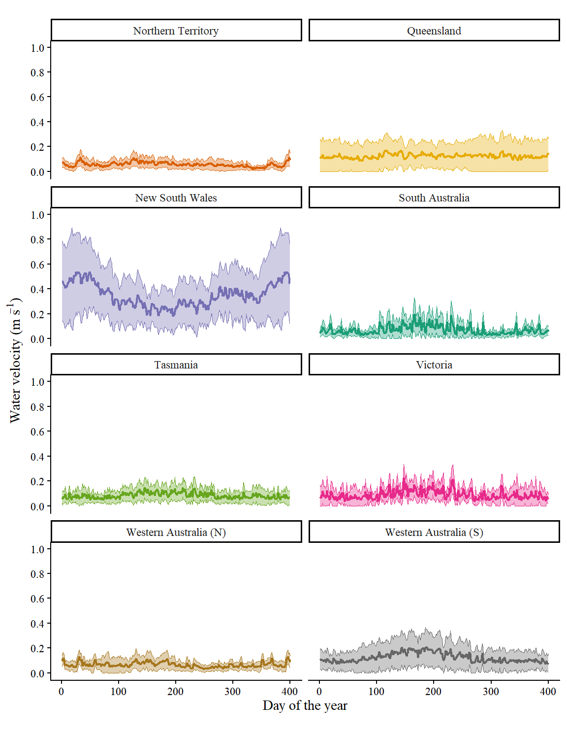
Figure 16
Code
stlims <- lims[lims$state == "WAN", ]

p_bathy %+% filter(cell_bathy, state == "WAN") +
  coord_sf(xlim = c(stlims$lonmin, stlims$lonmax), ylim = c(stlims$latmin, stlims$latmax), expand = F)
Coordinate system already present.
ℹ Adding new coordinate system, which will replace the existing one.
Figure 17
Code
stlims <- lims[lims$state == "WAS", ]

p_bathy %+% filter(cell_bathy, state == "WAS") +
  coord_sf(xlim = c(stlims$lonmin, stlims$lonmax), ylim = c(stlims$latmin, stlims$latmax), expand = F)
Coordinate system already present.
ℹ Adding new coordinate system, which will replace the existing one.
Figure 18

Extra stuff

Code
d_top_PL <- c(0.5, 1, 1.5, 2, 2.5, 3) # tar_read(d_top_PL, store = runs_store)

Ilim_cell <- runs_data %>% 
  list.files(full.names = T) %>% 
  str_subset("Ilim_cell") %>% 
  purrr::map_dfr(arrow::read_parquet)

# Ilim_means <- Ilim_cell %>% 
#   group_by(state, depth, yday) %>% 
#   reframe(I_lim = mean(I_lim, na.rm = T))
# 
# ggplot(Ilim_means, aes(x = yday, y = I_lim, colour = depth)) +
#   geom_line(linewidth = 0.75) +
#   facet_wrap(facets = vars(state)) +
#   theme_classic()

Ilim_means <- Ilim_cell %>% 
  group_by(state, depth) %>% 
  reframe(I_sd = sd(I_lim, na.rm = T),
          I_lim = mean(I_lim, na.rm = T))

ggplot(Ilim_means, aes(x = state, y = I_lim, fill = depth, ymin = I_lim-I_sd, ymax = I_lim+I_sd)) +
  geom_col(colour = "black", position = position_dodge(), width = 0.95) +
  geom_errorbar(position = position_dodge(width = 0.95), width = 0.5) +
  theme_classic()
Code
Ilim_cell <- Ilim_cell %>% 
  dplyr::filter(depth == "2.5") %>% 
  dplyr::select(-c(irradiance, depth, state)) %>% 
  merge(cell_coords, by = "cell_no")

# var_rast <- terra::rast(list(x = Ilim_cell$longitude, y = Ilim_cell$latitude, z = Ilim_cell$I_lim))
# crs(var_rast) <- "+proj=longlat +datum=WGS84 +ellps=WGS84 +towgs84=0,0,0"))