prettyplot2 <- prettyplot + theme(legend.position = "none", aspect.ratio = 0.75)
rm.x <- function(){theme(axis.text.x = element_blank(), axis.ticks.x = element_blank(), axis.title.x = element_blank())}
rm.y <- function(){theme(axis.text.y = element_blank(), axis.ticks.y = element_blank(), axis.title.y = element_blank())}

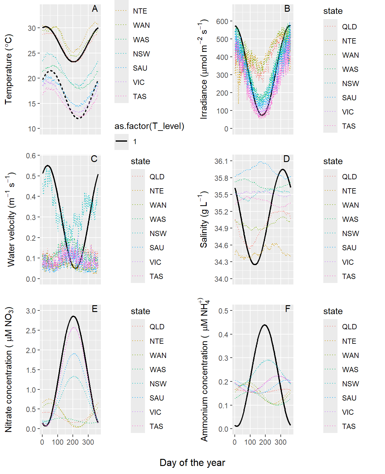
p1 <- sens_cond %>%
  dplyr::filter(t <= 365) %>%
  ggplot(aes(x = t, y = T_input, linetype = as.factor(T_level))) +
  geom_line(linewidth = 0.75) +
  geom_line(data = state_input_timeseries, aes(x = yday, y = T_input_mean, colour = state), linetype = "dotted", inherit.aes = F) +
  scale_y_continuous(breaks = seq(10, 35, 5), limits = c(10, 33.5)) +
  labs(y = expression("Temperature ("*degree*"C)")) +
  prettyplot2

p2 <- sens_cond %>%
  dplyr::filter(t <= 365 & T_level == 1) %>%
  ggplot(aes(x = t, y = I_input)) +
  geom_line(linewidth = 0.75) +
  geom_line(data = state_input_timeseries, aes(x = yday, y = I_input_mean, colour = state), linetype = "dotted", inherit.aes = F) +
  scale_y_continuous(breaks = seq(0, 700, 100), limits = c(0, 660)) +
  labs(y = expression("Irradiance ("*mu*"mol m"^-2*" s"^-1*")")) +
  prettyplot2

p3 <- sens_cond %>%
  dplyr::filter(t <= 365 & T_level == 1) %>%
  ggplot(aes(x = t, y = U_input)) +
  geom_line(linewidth = 0.75) +
  geom_line(data = state_input_timeseries, aes(x = yday, y = UV_input_mean, colour = state), linetype = "dotted", inherit.aes = F) +
  scale_y_continuous(breaks = seq(0, 0.6, 0.1), limits = c(0, 0.575)) +
  labs(y = expression("Water velocity (m"^-1*" s"^-1*")")) +
  prettyplot2

p4 <- sens_cond %>%
  dplyr::filter(t <= 365 & T_level == 1) %>%
  ggplot(aes(x = t, y = S_input)) +
  geom_line(linewidth = 0.75) +
  geom_line(data = state_input_timeseries, aes(x = yday, y = S_input_mean, colour = state), linetype = "dotted", inherit.aes = F) +
  scale_y_continuous(breaks = seq(33.1, 36.8, 0.3), limits = c(34, 36.11)) +
  labs(y = expression("Salinity (g L"^-1*")")) +
  prettyplot2

pdata1 <- sens_cond %>%
  dplyr::filter(t <= 365 & T_level == 1) %>%
  mutate(Ni_input = set_units(Ni_input, "mg m-3") %>% set_units("umol L-1") %>% drop_units(),
         Am_input = set_units(Am_input, "mg m-3") %>% set_units("umol L-1") %>% drop_units())
pdata2 <- state_input_timeseries %>%
  mutate(Ni_input_mean = set_units(Ni_input_mean, "mg m-3") %>% set_units("umol L-1") %>% drop_units(),
         Am_input_mean = set_units(Am_input_mean, "mg m-3") %>% set_units("umol L-1") %>% drop_units())

p5 <- pdata1 %>%
  ggplot(aes(x = t, y = Ni_input)) +
  geom_line(linewidth = 0.75) +
  geom_line(data = pdata2, aes(x = yday, y = Ni_input_mean, colour = state), linetype = "dotted", inherit.aes = F) +
  scale_y_continuous(breaks = seq(0, 5, 0.5), limits = c(0, 3)) +
  labs(y = nitrate_lab) +
  prettyplot2

p6 <- pdata1 %>%
  ggplot(aes(x = t, y = Am_input)) +
  geom_line(linewidth = 0.75) +
  geom_line(data = pdata2, aes(x = yday, y = Am_input_mean, colour = state), linetype = "dotted", inherit.aes = F) +
  scale_y_continuous(breaks = seq(0, 10, 0.1), limits = c(0, 0.5)) +
  labs(y = ammonium_lab) +
  prettyplot2

plot_grid(
  plot_grid(
    p1 + rm.x() + annotate("text", x = Inf, y = Inf, label = "A", hjust = 1.5, vjust = 1, size = 4, fontface = "plain"),
    p2 + rm.x() + annotate("text", x = Inf, y = Inf, label = "B", hjust = 1.5, vjust = 1, size = 4, fontface = "plain"),
    p3 + rm.x() + annotate("text", x = Inf, y = Inf, label = "C", hjust = 1.5, vjust = 1, size = 4, fontface = "plain"),
    p4 + rm.x() + annotate("text", x = Inf, y = Inf, label = "D", hjust = 1.5, vjust = 1, size = 4, fontface = "plain"),
    p5 + theme(axis.title.x = element_blank()) +
      annotate("text", x = Inf, y = Inf, label = "E", hjust = 1.5, vjust = 1, size = 4, fontface = "plain"),
    p6 + theme(axis.title.x = element_blank()) +
      annotate("text", x = Inf, y = Inf, label = "F", hjust = 1.5, vjust = 1, size = 4, fontface = "plain"),
    ncol = 2, align = "hv"
  ),
  ggdraw() + draw_label("Day of the year", size = 12),
  ncol = 1,
  rel_heights = c(0.95, 0.05)
)