Results: Ambient growth limitations

Modelling Asparagopsis nitrogen bioremediation efficiency in Australian coastal environments

Author

Tormey Reimer

Published

5 August 2026

Load in all the BARRA-R2 cells being used, with their coordinates.
cell_coords <- find_read(envi_data, "R2_cell_coords") %>% 
  mutate(state = factor(state, levels = states_ord)) %>% 
  dplyr::select(-layer)
cells_included <- find_read(runs_data, "include")
cells_omitted <- find_read(runs_data, "omit")

totals <- cell_coords %>% 
  filter(!cell_no %in% cells_omitted) %>% 
  group_by(state) %>% 
  reframe(cells = n())

The point of this section is to show the most common limiting factor - overall, between species, temporally, geographically.

Code
# These have cell_no, lat, lon, month and lims (for maps)
armata_lims <- map(1:12, function(m) {
  file.path(runs_data, str_c("armata_dom_lims_raster_", fixnum(m,2), ".tif")) %>% 
    terra::rast() %>% 
    as.data.frame(xy=TRUE) %>% 
    rename(longitude = x, latitude = y) %>% 
    mutate(lim = factor(lim, levels = 1:4, labels = c("T_lim", "I_lim", "Q_lim", "S_lim")))
  })
taxiformis_lims <- map(1:12, function(m) {
  file.path(runs_data, str_c("taxiformis_dom_lims_raster_", fixnum(m,2), ".tif")) %>% 
    terra::rast() %>% 
    as.data.frame(xy=TRUE) %>% 
    rename(longitude = x, latitude = y) %>% 
    mutate(lim = factor(lim, levels = 1:4, labels = c("T_lim", "I_lim", "Q_lim", "S_lim")))
  })

# These have only latitude, month and lim (for histograms)
forhist_armata <- find_read(runs_data, "forhist_armata.parquet") %>% split(.$month)
forhist_taxiformis <- find_read(runs_data, "forhist_taxiformis.parquet") %>% split(.$month)
Code
p_dom_hist.1 <- forhist_armata[[1]] %>% 
  ggplot(aes(y = latitude, x = after_stat(100*count/(13207 * 30)), fill = lim, colour = lim)) +
  geom_histogram(position = "stack", alpha = 0.75, binwidth = 0.75) +
  scale_fill_manual(values = lims_pal) +
  scale_colour_manual(values = lims_pal) +
  scale_y_continuous(limits = c(-44.5, -8.5), expand = c(0,0)) +
  scale_x_continuous(limits = c(0, 5.5), breaks = seq(0, 5, 1), expand = c(0.02,0)) +
  labs(x = expression("% of growing days in all cells"), y = "Latitude") +
  prettyplot() +
  rm.y() + 
  theme(plot.margin = margin(0, 0, 0, 0, "pt"), panel.spacing = unit(1, "lines"))

p_dom_map.1 <- armata_lims[[1]] %>% 
  ggplot(aes(x = longitude, y = latitude, fill = lim)) +
  geom_raster() +
  geom_sf(data = ozmap_data(data = "states"), inherit.aes = F) +
  coord_sf(xlim = c(111.5, 155), ylim = c(-44.5, -8.5), expand = F) +
  scale_x_continuous(breaks = seq(112.5, 160, 10)) +
  scale_y_continuous(breaks = seq(-2.5, -45, -5)) +
  scale_color_brewer(palette = "Dark2") +
  scale_fill_manual(values = lims_pal) +
  labs(x = "Longitude", y = "Latitude") +
  prettyplot() + 
  theme(plot.margin = margin(0, 0, 0, 0, "pt"), axis.title.x = element_text(vjust = 1))

Asparagopsis armata

Code
stat1 <- armata_lims %>% 
  filter(latitude > -30) 
stat1 <- stat1 %>% 
  group_by(cell_no, lim) %>% 
  reframe(perc_days = n()/nrow(stat1))
stat1_T <- sum(stat1$perc_days[stat1$lim == "T_lim"])
stat1_Q <- sum(stat1$perc_days[stat1$lim == "Q_lim"])
stat1_I <- sum(stat1$perc_days[stat1$lim == "I_lim"])

stat2 <- armata_lims %>% 
  filter(latitude <= -30)
stat1 <- stat1 %>% 
  group_by(cell_no, lim) %>% 
  reframe(perc_days = n()/nrow(stat1))
stat2_T <- sum(stat2$perc_days[stat2$lim == "T_lim"])
stat2_Q <- sum(stat2$perc_days[stat2$lim == "Q_lim"])
stat2_I <- sum(stat2$perc_days[stat2$lim == "I_lim"])

# For _A. armata_ grown at latitudes > -30$^\circ$, a mean of
# `r round(100*stat1_T,1)`% of growing days were limited by temperature,
# `r round(100*stat1_Q,1)`% were limited by nutrients, and
# `r round(100*stat1_I,1)`% were limited by light.
# 
# For _A. armata_ grown at latitudes < -30$^\circ$, a mean of
# `r round(100*stat2_T,1)`% of growing days were limited by temperature,
# `r round(100*stat2_Q,1)`% were limited by nutrients, and
# `r round(100*stat2_I,1)`% were limited by light.

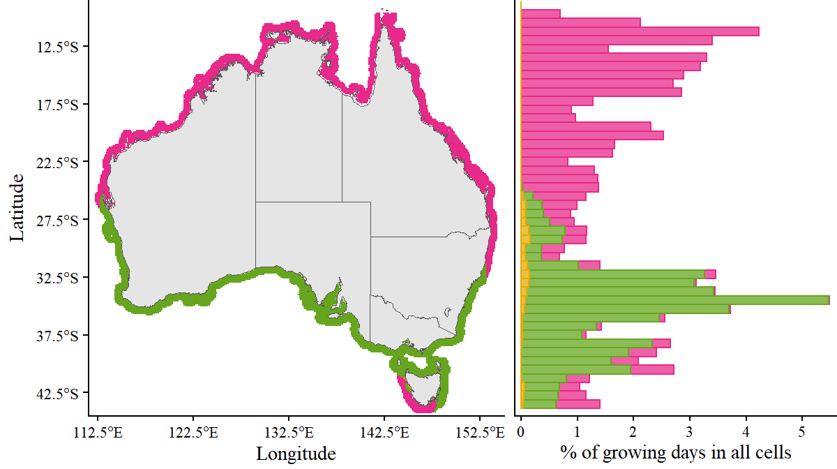
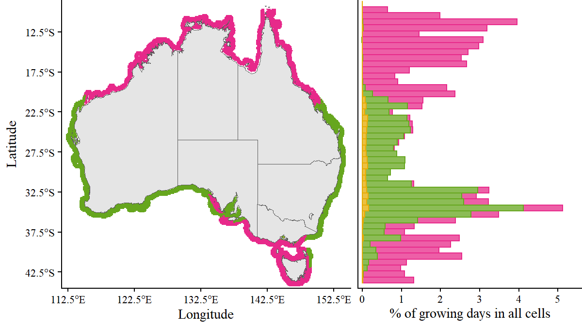
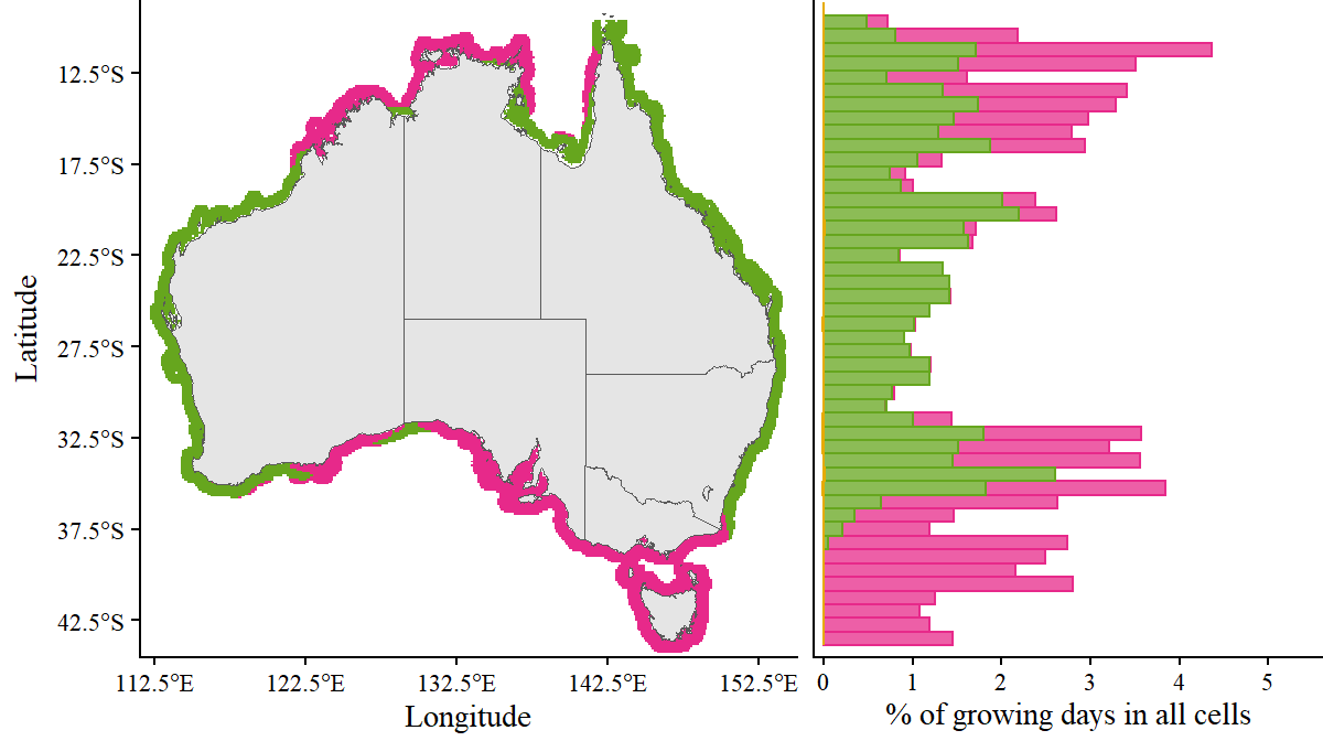
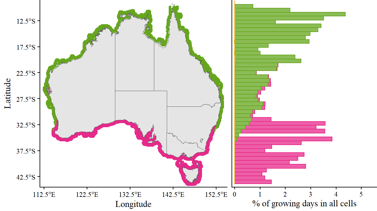
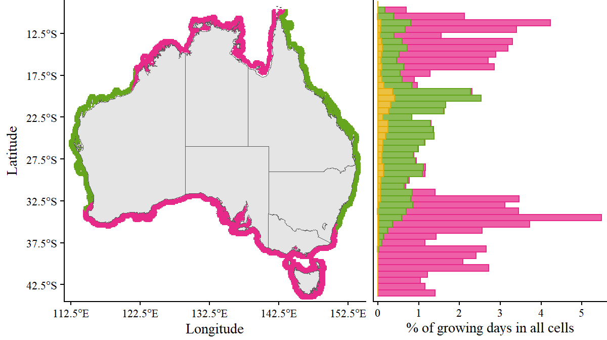
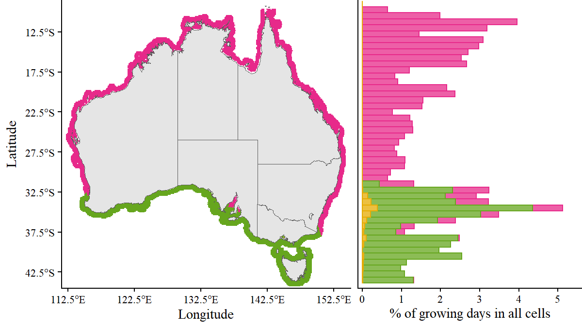
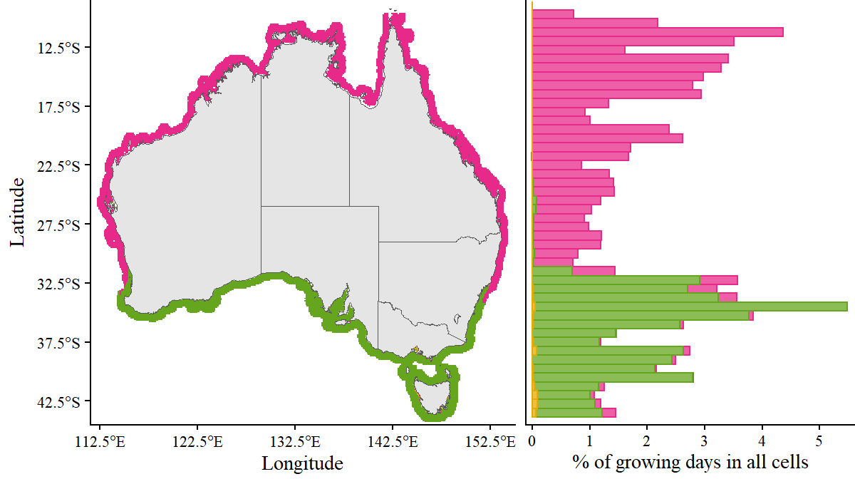
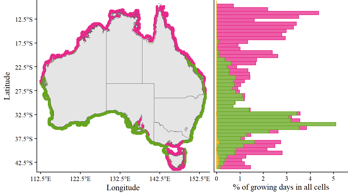
Factors limiting growth of A. armata in February (A), May (B), August (C) and November (D). Colours indicate limiting factors as temperature (pink), internal nutrient quotient (green) or light availability (gold). Maps show the dominant limiting factor in each cell within the month, while historgram shows the frequency of limiting factors across all days of the month in all cells.
Code
plot_grid(
  p_dom_map.1 %+% armata_lims[[2]],
  p_dom_hist.1 %+% forhist_armata[[2]],
  ncol = 2, 
  align = "h", 
  rel_widths = c(1, 0.625)
)  
Warning: <ggplot> %+% x was deprecated in ggplot2 4.0.0.
ℹ Please use <ggplot> + x instead.
Warning: Removed 6 rows containing missing values or values outside the scale range
(`geom_bar()`).
Code
plot_grid(
  p_dom_map.1 %+% armata_lims[[5]],
  p_dom_hist.1 %+% forhist_armata[[5]],
  ncol = 2, 
  align = "h", 
  rel_widths = c(1, 0.625)
)
Warning: Removed 7 rows containing missing values or values outside the scale range
(`geom_bar()`).
Code
plot_grid(
  p_dom_map.1 %+% armata_lims[[8]],
  p_dom_hist.1 %+% forhist_armata[[8]],
  ncol = 2, 
  align = "h", 
  rel_widths = c(1, 0.625)
)
Warning: Removed 7 rows containing missing values or values outside the scale range
(`geom_bar()`).
Code
plot_grid(
  p_dom_map.1 %+% armata_lims[[11]],
  p_dom_hist.1 %+% forhist_armata[[11]],
  ncol = 2, 
  align = "h", 
  rel_widths = c(1, 0.625)
)
Warning: Removed 6 rows containing missing values or values outside the scale range
(`geom_bar()`).
Figure 1
Figure 2
Figure 3
Figure 4

Asparagopsis taxiformis

Code
stat1 <- taxiformis_lims %>% 
  filter(latitude > -30) 
stat1 <- stat1 %>% 
  group_by(cell_no, lim) %>% 
  reframe(perc_days = n()/nrow(stat1))
stat1_T <- sum(stat1$perc_days[stat1$lim == "T_lim"])
stat1_Q <- sum(stat1$perc_days[stat1$lim == "Q_lim"])
stat1_I <- sum(stat1$perc_days[stat1$lim == "I_lim"])

stat2 <- taxiformis_lims %>% 
  filter(latitude <= -30)
stat1 <- stat1 %>% 
  group_by(cell_no, lim) %>% 
  reframe(perc_days = n()/nrow(stat1))
stat2_T <- sum(stat2$perc_days[stat2$lim == "T_lim"])
stat2_Q <- sum(stat2$perc_days[stat2$lim == "Q_lim"])
stat2_I <- sum(stat2$perc_days[stat2$lim == "I_lim"])

# For _A. taxiformis_ grown at latitudes > -30$^\circ$, a mean of
# `r round(100*stat1_T,1)`% of growing days were limited by temperature,
# `r round(100*stat1_Q,1)`% were limited by nutrients, and
# `r round(100*stat1_I,1)`% were limited by light.
# 
# For _A. taxiformis_ grown at latitudes < -30$^\circ$, a mean of
# `r round(100*stat2_T,1)`% of growing days were limited by temperature,
# `r round(100*stat2_Q,1)`% were limited by nutrients, and
# `r round(100*stat2_I,1)`% were limited by light.

Factors limiting growth of A. taxiformis in February (A), May (B), August (C) and November (D). Colours indicate limiting factors as temperature (pink), internal nutrient quotient (green) or light availability (gold). Maps show the dominant limiting factor in each cell within the month, while historgram shows the frequency of limiting factors across all days of the month in all cells.
Code
plot_grid(
  p_dom_map.1 %+% taxiformis_lims[[2]],
  p_dom_hist.1 %+% forhist_taxiformis[[2]],
  ncol = 2, 
  align = "h", 
  rel_widths = c(1, 0.625)
)  
Warning: Removed 6 rows containing missing values or values outside the scale range
(`geom_bar()`).
Code
plot_grid(
  p_dom_map.1 %+% taxiformis_lims[[5]],
  p_dom_hist.1 %+% forhist_taxiformis[[5]],
  ncol = 2, 
  align = "h", 
  rel_widths = c(1, 0.625)
)  
Warning: Removed 7 rows containing missing values or values outside the scale range
(`geom_bar()`).
Code
plot_grid(
  p_dom_map.1 %+% taxiformis_lims[[8]],
  p_dom_hist.1 %+% forhist_taxiformis[[8]],
  ncol = 2, 
  align = "h", 
  rel_widths = c(1, 0.625)
)  
Warning: Removed 7 rows containing missing values or values outside the scale range
(`geom_bar()`).
Code
plot_grid(
  p_dom_map.1 %+% taxiformis_lims[[11]],
  p_dom_hist.1 %+% forhist_taxiformis[[11]],
  ncol = 2, 
  align = "h", 
  rel_widths = c(1, 0.625)
)  
Warning: Removed 6 rows containing missing values or values outside the scale range
(`geom_bar()`).
Figure 5
Figure 6
Figure 7
Figure 8